Transfer Learning: Standing on the Shoulders of Giants

This repository holds a quick demo of a practical use of the concepts in this article.
While trying to solve a machine learning proble, most of us pass through an iterative process in which, after the data collection and analysis tasks, we try different preprocessing and different models to optimize a certain metric, either the crossentropy loss for a classification model or the Huber loss in a regression model, for example.
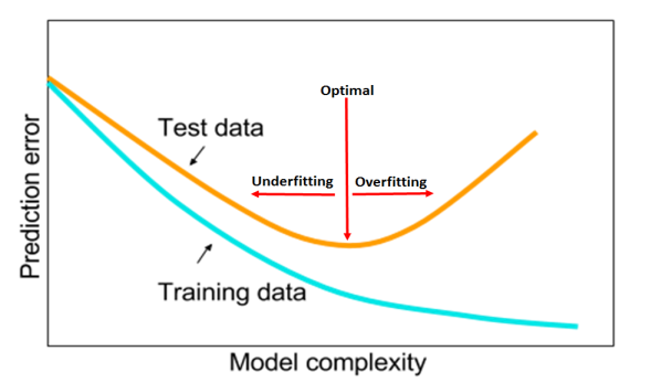
On that process, a cycle of underfitting and overfitting is often repeated. In this cycle the first phase is often characterized by our models not being sufficiently complex to capture the different patterns of the data, followed by a phase when we make them too complex and we make them learn specific features of the training set instead of general features and characteristics that could be used in a different dataset.

Regularization techniques such as Dropout or L2 regularization can help us solve the problem of overfitting, as they penalize the complexity of the model. The implementation of these methods is often recommended above the restriction of units per layer or the number of layers, as they are prepared to let those important parameters to compensate for the loss added to the model.
Nevertheless, no matter how many regularization we use we eventually end up facing a barrier that we cannot overcome: The scarce volume of data we have. Even if we try to help our models, they only learn what is present in the training set, and if the training set is small or its diversity is not enough our models will eventually fail. In the end, they need to reduce a certain metric as much as possible, and they will adapt to the data whenever possible, so either we make them adapt too much (overfitting) to reduce the training loss, or too little (underfitting) to reduce the discrepancy between the training and validation losses.
To help with this problem, we can use data augmentation. For example, if we were to use Keras to train a model, we could use the ImageDataGenerator to create synthetic data from the training set, and use it to train our model.
from tensorflow.keras.preprocessing.image import ImageDataGenerator

datagen = ImageDataGenerator(
      rotation_range=40,
      width_shift_range=0.2,
      height_shift_range=0.2,
      shear_range=0.2,
      zoom_range=0.2,
      horizontal_flip=True,
      fill_mode='nearest'
)
Here we can see how using parameters as horizontal_flip we could create a new image from another one by rotating it over its Y axis, which would imply giving our model an example more for capturing those generic patterns that we commented before.
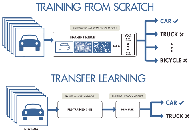
Although, this type of techniques end up using our training set as well, so if this is very poor, we will not be able to solve our problem. In this case, wouldn’t it be great to import a model trained by another person in a better dataset, with a better architecture? Enter Transfer Learning.
Transfer Learning

By using public available model repositories such as Tensorflow Hub we can access pre-trained models and download them for use in our notebooks. In addition, well known models as GloVe or VGG16 have functions inside their own modules in Keras that we can access in order to load various implementations of those models.
from tensorflow.keras.applications import VGG16

conv_base = VGG16(
    weights='imagenet',
    include_top=False,
    input_shape=(150, 150, 3)
)

# Shows the structure of the convnet
conv_base.summary()

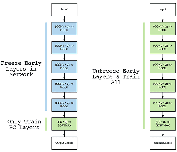
# Freezing the layers so they don't get modified at training
conv_base.trainable = False
This step load the first layers (often called the body of the network) of the VGG16 model, as the last layers (those usually called the head) are specific for each task, as they are the ones in charge of classifying the input images in the different classes. In this case, adding a classifier over the pretrained model would be easy, and would allow us to train our model together using the same methods we would use with a model conceived completely by us:
from tensorflow.keras.models import Sequential
from tensorflow.keras.layers import Dense, Flatten, Dropout

model = Sequential([
    conv_base,
    Flatten(),
    Dense(256, activation='relu', kernel_regularizer=l2(0.001)),
    Dropout(0.3),
    Dense(128, activation='relu', kernel_regularizer=l2(0.001)),
    Dropout(0.3),
    Dense(2, activation='softmax'),
])

model.compile(
    optimizer='rmsprop',
    loss='categorical_crossentropy',
    metrics=['accuracy']
)

history = model.fit(
    train_generator,
    steps_per_epoch=1000,
    epochs=10,
    validation_data=validation_generator,
    validation_steps=250,
)
Fine Tuning
The performance of our model at this point would have increased by a large margin, as using a model which already knew the general patterns of the images presented would have saved us tons of time and effort. We were able to tune the model by simply adding a head block on top of the pretrained model, but what happens if we start having more and more data or if the pretrained model does not fit our needs? In those cases we could apply Fine Tuning to further adjust the pretrained model so it can perform better in our particular task.

Fine Tuning is based on the idea of unfreeze the last layers of the model (those which encapsulate more specific patterns and features) and then train our model in our specific problem, so their weights get more adequate to the task at hand. We should consider that this is a risky practice, as if we modify the weights without being sure that the quality of our training set is adequate, we could end up making our model worse or even falling under the Catastrophic Forgetting problem. Nevertheless, it is worth a try and very advisable when we know at which extend to use it. As a rule of thumb, avoid modifying the first layers of a pretrained model, and use a small learning rate while fine tuning.
Keras offers a very friendly interface to do this in the last layers, as we can see in this snippet inspired in the book Deep Learning with Python from François Chollet:
conv_base = VGG16(
    weights='imagenet',
    include_top=False,
    input_shape=(150, 150, 3)
)

set_trainable = False
for layer in conv_base.layers:
    if layer.name == 'block5_conv1':
        set_trainable = True
    if set_trainable:
        layer.trainable = True
    else:
        layer.trainable = False
After the modification of the body of the model, in this case called convbase, we can add a head block as before so its weights will be adjusted during the training process as well.
In the particular case of the repository listed at the top of this page, we can see that on the Dogs vs Cats dataset the accuracy of the model is improved from 81% of precision to 90% thanks to the use of the Transfer Learning technique. Furthermore, we went even further as, thanks to the fine tuning of our model, we obtained an accuracy of 95% of precision. This may be a good proof of how easy is to use Transfer Learning in a small project, where the access to the data is expensive or impossible, so it is one of the best tools to have in your hands while working on a personal project.
Thank you very much for your attention and keep on learning!